Examples

import matplotlib.pyplot as plt
import networkx as nx
import numpy as np

To get started, we essentially need two things:

• A graph construction method (see Graph construction)

• A construction method for the conditionals (see Conditionals)

from bn_testing.models import BayesianNetwork
from bn_testing.dags import ErdosReny
from bn_testing.conditionals import PolynomialConditional

model = BayesianNetwork(
    n_nodes=20,
    dag=ErdosReny(p=0.1),
    conditionals=PolynomialConditional(max_terms=2),
    random_state=20)

model.show()

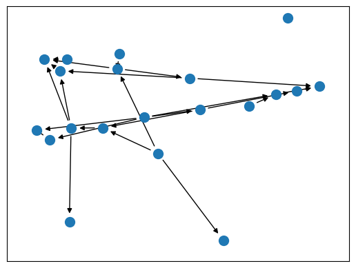
After the model has been generated, all transformations have been stored in model.transformations:

{
  'f00': 8.1*f01^5 + -9.7*f01^5,
  'f01': -8.9*f10^5 + -1.6*f10^5,
  'f02': 4.6*f19^5 + 3.8*f19^5,
  'f03': -9.9*f05^2 + -8.6*f05^2,
  'f05': -9.4*f12^7 + 3.2*f12^7,
  'f06': -3.8*f05^6*f02^2,
  'f08': -7.1*f10^2*f04^1 + -9.4*f10^1*f04^2,
  'f09': -7.2*f19^2*f05^1*f07^1*f06^1 + 3.7*f19^1*f05^2*f07^1*f06^1
  'f12': 6.5*f16^3*f01^1 + 6.2*f16^1*f01^3,
  'f13': 6.7*f16^4,
  'f15': 9.6*f08^1*f00^7*f02^4,
  'f17': -5.5*f10^6,
  'f18': -9.3*f10^4*f17^2,
  'f19': -2.7*f16^7*f14^4,
}

Sampling

df = model.sample(10000)

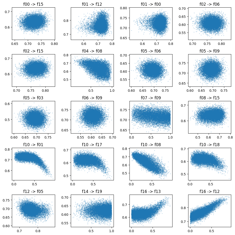
Edge scatters

fig, axes = plt.subplots(figsize=(10, 10), ncols=4, nrows=5)

for edge, ax in zip(model.edges, axes.ravel()):
    ax.scatter(df[edge[0]], df[edge[1]], alpha=0.2, s=2)
    ax.set_title(f"{edge[0]} -> {edge[1]}")

fig.tight_layout()

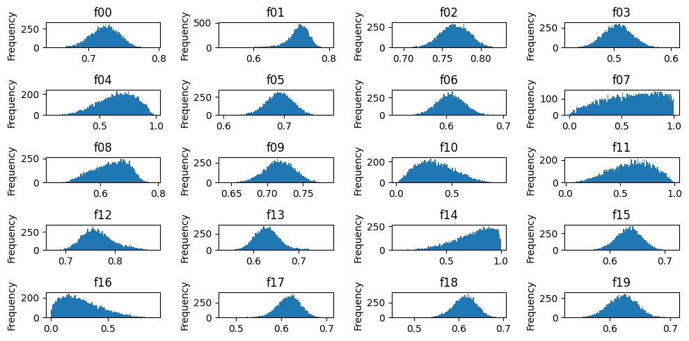
Marginal distributions

fig, axes = plt.subplots(figsize=(10, 5), ncols=4, nrows=5)

for ax, c in zip(axes.ravel(), df.columns):
    df[c].plot.hist(ax=ax, bins=100)
    ax.set_title(c)
fig.tight_layout()

Saving and loading

A model object can be saved to disk as follows:

model.save('/path/to/model.pkl')

Afterwards, it can be loaded using:

from bn_testing.models import BayesianNetwork
model = BayesianNetwork.load('/path/to/model.pkl')